GSW13: 3rd Generation Homomorphic Encryption from Learning with Errors

This week our reading group studied Homomorphic Encryption from Learning with Errors: Conceptually-Simpler, Asymptotically-Faster, Attribute-Based by Craig Gentry, Amit Sahai and Brent Waters: a 3rd generation fully homomorphic encryption scheme.

The paper is partly motivated by that multiplication in previous schemes was complicated or at least not natural. Let’s take the BGV scheme where ciphertexts are simply LWE samples for and with being the message bit and is some “small” error. Let’s write this as because it simplifies some notation down the line. In this notation, multiplication can be accomplished by because . However, we now need to map back to using “relinearisation”, this is the “unnatural” step.

However, this is only unnatural in this particular representation. To see this, let’s rewrite as a linear multivariate polynomial . This polynomial evaluates to on the secret . Note that evaluating a polynomial on is the same as reducing it modulo the set of polynomials .

Now, multiplying produces a quadratic polynomial. Its coefficients are produced from all the terms in the tensor product . In other words, the tensor product is just another way of writing the quadratic polynomial . Evaluating on evaluates to . To map this operation to note that evaluating on is the same as taking the inner product of vector of coefficients of and the vector . For example, evaluating at and is the same as taking the inner product of and . That is, if we precompute all the products up to degree two of and the remaining operations are just an inner product.

Still, is a quadratic polynomial, we’d want a linear polynomial. In BGV this reduction is referred to as “relinearisation” (which is not helpful if you’re coming from a commutative algebra background). Phrased in terms of commutative algebra, what we’re doing is to reduce modulo elements in the ideal generated by .

Let’s look at what happens when we reduce by some element in the ideal generated by . We start with the leading term of which is . To reduce this term we’d add to , which is an element in the ideal generated by since it is a multiple of . This produces which has a smaller leading term. Now, we’d add the appropriate element with leading term and so on.

Of course, this process, as just described, assumes access to which is the same as giving out our secret . Instead, we want to precompute multiples with leading terms , and and publish those. This is still insecure, but adding some noise, assuming circular security and doing a bit more trickery we can make this as secure as the original scheme. This is then what “relinearisation” does. There is also an issue with noise blow up, e.g. multiplying a sample by a scalar like makes its noise much bigger. Hence, we essentially publish elements with leading terms , , , , , , , , , and so on, which allows us to avoid those multiplications. Before I move on to GSW13 proper, I should note that all this has been pointed out in 2011.

The Scheme

Ciphertexts in the GSW13 scheme are matrices over with entries. The secret key is a vector of dimensions over with at least one big coefficient . Let’s restrict . We say that encrypts when for some small . To decrypt we simply compute and check if there are large coefficients in .

Ciphertexts in fully homomorphic encryption schemes are meant to be added and multiplied. Starting with addition, consider . We have

Moving on to multiplication, we first observe that if matrices and have a common exact eigenvector with eigenvalues and , then their product has eigenvector with eigenvalue . But what about the noise?

Considering :

1. 
2. 
3. 
4. 
5. 
6. 

In the above expression , , , are all small, is not. In other words, the signal is not drowned by the noise and we have achieved multiplication. How far can we go with this, though?

Multiplicative Depth

Assume , , are all in absolute value. After multiplication is bounded by . Hence, if we have levels, the noise grows worse than . We require , otherwise the wrap-around will kill us. Also, must be sub-exponential in for security reasons. The bigger this gap, the easier the lattice problem we are basing security on and if the gap is exponential then there is a polynomial-time algorithm for solving this lattice problem: the famous LLL algorithm. As a consequence, the scheme as-is allows to evaluate polynomials of degree sublinear in .

To improve on this, we need a new notion. We call strongly bounded if the entries of are bounded by 1 and the error is bounded by .

In what follows, we will only consider a NAND gate: . NAND is a universal gate, so we can build any circuit with it. However, in this context its main appeal is that it ensures that the messages stay . Note the term above which is big if is big. If and are strongly bounded then error vector of is bounded by instead of . Now, If we could make the entries of bounded by 1 again, itself would be strongly bounded and we could repeat the above argument. In other words, this would enable circuits of depth , i.e. polynomial depth circuits (instead of merely polynomial degree) when is sub-exponential as above.

Flatten

We’ll make use of an operation BitDecomp which splits a vector of integers into a longer vector of the bits of the integers. For example, becomes which has length . Here’s a simple implementation in Sage:

def bit_decomp(v):
    R = v.base_ring()
    k = ZZ((R.order()-1).nbits())
    w = vector(R, len(v)*k)
    for i in range(len(v)):
        for j in range(k):
            if 2**j & ZZ(v[i]):
                w[k*i+j] = 1
            else:
                w[k*i+j] = 0
    return w

We also need a function which reverses the process, i.e. adds up the appropriate powers of two: . It is called in the GSW13 paper, but I’ll simply call it … BitComp.

def bit_comp(v):
    R = v.base_ring()
    k = ZZ((R.order()-1).nbits())
    assert(k.divides(len(v)))
    w = vector(R, len(v)//k)
    for i in range(len(v)//k):
        for j in range(k):
            w[i] += 2**j * ZZ(v[k*i+j])
    return w

Actually, the definition of BitComp is a bit more general than just adding up bits. As defined above — following the GSW13 paper — it will add up any integer entry of multiplied with the appropriate power of two multiplied in. This is relevant for the next function we define, namely Flatten which we define as BitDecomp(BitComp(⋅)).

flatten = lambda v: bit_decomp(bit_comp(v))

Finally we also define PowersOf2 which produces a new vector from as :

def powers_of_two(v):
    R = v.base_ring()
    k = ZZ((R.order()-1).nbits())
    w = vector(R, len(v)*k)
    for i in range(len(v)):
        for j in range(k):
            w[k*i+j] = 2**j * v[i]
    return w

For example the output of PowersOf2 on for is . Having defined these functions, let’s look at some identities. It holds that

which can verified by recalling integer multiplication. For example, . Another example: and

Or in the form of some Sage code:

q = 8
R = IntegerModRing(q)
v = random_vector(R, 10)
w = random_vector(R, 10)
v.dot_product(w) == bit_decomp(v).dot_product(powers_of_two(w))

Furthermore, let be an dimensional vector and be a dimensional vector. Then it holds that

because .

Finally, we have

by combining the previous two statements.

For example, let , , .

1. BitComp on gives
2. BitDecomp on gives ,
3. For the left-hand side we have .
4. For the right-hand side we hve .

The same example in Sage:

q = 8
R = IntegerModRing(q)
a = vector(R, (2,3,0))
b = vector(R, (3,))

bit_comp(a).dot_product(b) == flatten(a).dot_product(powers_of_two(b))

Hence, running Flatten on produces a strongly bounded matrix . Boom.¹

Key Generation

It remains to sample a key and to argue why this construction is secure if LWE is secure for the choice of parameters.

To generate a public key, pick LWE parameters and and sample as usual.

The secret key is of dimension . The public key is , where we roll into , which now has dimension .

To encrypt, sample an matrix with entries and compute which is an matrix. That is, we do exactly what we would do with Regev’s original public-key scheme based on LWE: doing random linear combinations of the rows of to make fresh samples. Run BitDecomp on the output to get a matrix. Finally, set

For correctness, observe:

1. 
2. 
3. + something small.

The security argument is surprisingly simple. Consider . Because is already the output of Flatten it reveals nothing more than .

Unpacking 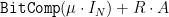to , note that is statistically uniform by the leftover hash lemma for uniform . Finally, is indistinguishable from a uniform by the decisional LWE assumption. Boom.

You promised 3rd Generation

So far, this scheme is not more efficient than previous ring-based schemes such as BGV, even asymptotically. However, an observation by Zvika Brakerski and Vinod Vaikuntanathan in Lattice-Based FHE as Secure as PKE changed this. This observation is that the order of multiplications matters. Let’s multiply four ciphertexts .

The traditional approach would be:

1. ,
2. 
3. 

In this approach the noise grows as follows:

1. 
2. 
3. 
4. 
5. 

Note the factor. That is, for multiplications we get a noise of size .

In contrast, consider this sequential approach:

1. ,
2. 
3. 

Under this order, the noise grows as:

1. 
2. 
3. 
4. 
5. 
6. 
7. 

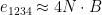
Note that each matrix is mutliplied by some only. Hence, here the noise grows linearly in number of multiplications i.e. as .

Footnotes:

¹

I suggest people start writing Boom instead of qed.